Forward Model

Single Spot

Perhaps the best way to learn how dot works is to experiment with it, which we will do in this tutorial. Let’s suppose first we have a star with a single spot, defined its latitude, longitude, and radius. We’ll place the star on the prime meridian (zero point in longitude) and the equator. We’ll give the star a rotation period of 0.5 days, and the spot will have contrast 0.3. To do this, we’ll first need to generate an instance of the Model object:

import pymc3 as pm
import numpy as np
from lightkurve import LightCurve

from dot import Model

times = np.linspace(-1, 1, 1000)
fluxes = np.zeros_like(times)
errors = np.ones_like(times)

rotation_period = 0.5  # days
stellar_inclination = 90  # deg

m = Model(
    light_curve=LightCurve(times, fluxes, errors),
    rotation_period=rotation_period,
    n_spots=1,
    contrast=0.3
)

Now that our Model is specified and the time points are defined in the LightCurve object, we can specify the spot properties:

# Create a starting point for the dot model
start_params = {
    "dot_R_spot": np.array([0.1]),
    "dot_lat": np.array([np.pi/2]),
    "dot_lon": np.array([0]),
    "dot_comp_inc": np.radians(90 - stellar_inclination),
    "dot_ln_shear": -3,
    "dot_P_eq": rotation_period,
    "dot_f0": 1
}

# Need to call this to validate ``start``
pm.util.update_start_vals(start, m.pymc_model.test_point, m.pymc_model)

We specify spot properties with a dictionary which contains the spot radii, latitudes, longitudes, the complementary angle to the stellar inclination, the natural log of the shear rate, the equatorial rotation period and the baseline flux of the star. We then call update_start_vals on the dictionary with our Model object, which translates the user-facing, human-friendly coordinates into the optimizer-friendly transformed coordinates.

We can now call our model on the start dictionary, and plot it like so:

import matplotlib.pyplot as plt

forward_model_start = m(start_params)

plt.plot(m.lc.time[m.mask], m.lc.flux[m.mask], m.lc.flux_err[m.mask],
         color='k', fmt='.', ecolor='silver')
plt.plot(m.lc.time[m.mask][::m.skip_n_points], forward_model_start,
         color='DodgerBlue')
plt.show()

(Source code, png, hires.png, pdf)

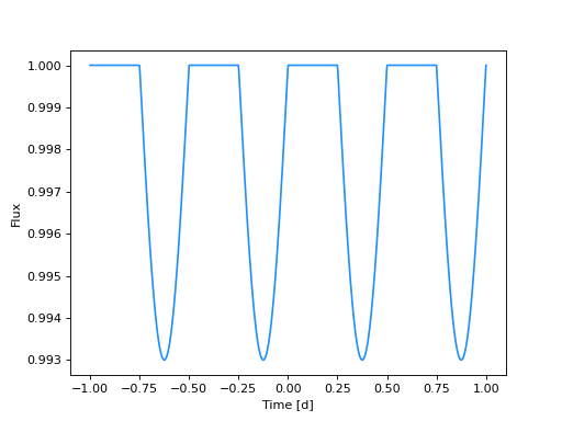
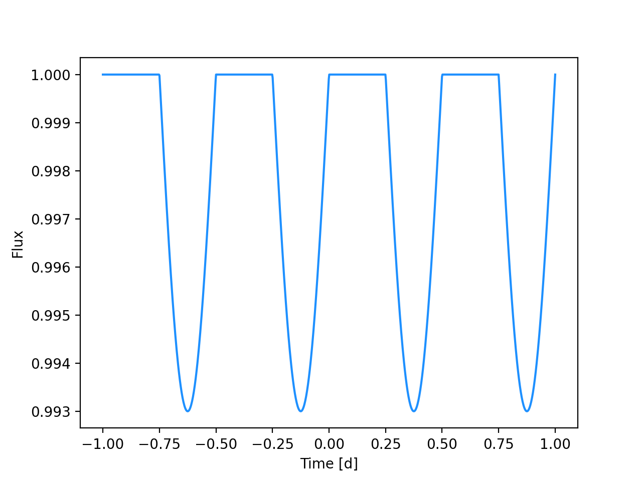
In the above plot, we see the forward model for the spot modulation of a single spot on a rotating star.

Differentially rotating spots

The syntax is similar for multiple spots, we just add extra elements to the numpy arrays which determine the spot parameters, like so:

m = Model(
    light_curve=LightCurve(times, fluxes, errors),
    rotation_period=rotation_period,
    n_spots=2,
    contrast=0.3
)

# Create a starting point for the dot model
two_spot_params = {
    "dot_R_spot": np.array([[0.1, 0.05]]),
    "dot_lat": np.array([[np.pi/2, np.pi/4]]),
    "dot_lon": np.array([[0, np.pi]]),
    "dot_comp_inc": np.radians(90 - stellar_inclination),
    "dot_ln_shear": np.log(0.2),
    "dot_P_eq": rotation_period,
    "dot_f0": 1
}

Note this time that we’ve set the shear rate to 0.2, which is the solar shear rate. This time when we plot the result we’ll see a more complicated model:

(Source code, png, hires.png, pdf)

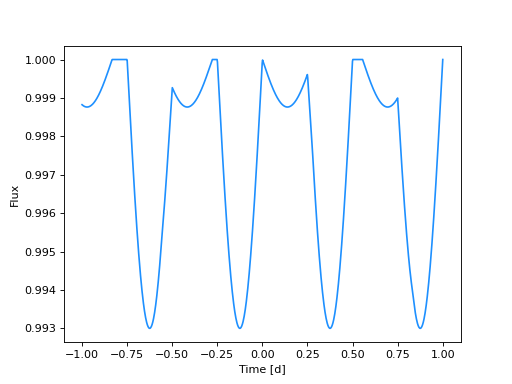
Now you can see the effect of differential rotation on the light curve – the smaller, higher latitude spot is rotating around the stellar surface with a different rate than the large, equatorial spot.