Getting Started
Note
If you plan to copy and paste the code in this tutorial into a notebook,
no modifications are needed to run the examples. However, if you run it in
from a Python script (.py file), you need to add the following line
if __name__ == "__main__": to the top of the code or else you’ll hit a
RuntimeError.
Load a light curve
dot uses LightCurve objects to handle light curves.
For quick and easy access to an example light curve, we include the light curve
of AB Doradus in the package, which you can access with:
import numpy as np
import matplotlib.pyplot as plt
from dot import ab_dor_example_lc
min_time = 0
max_time = 2
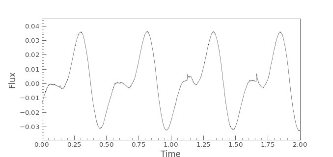
lc = ab_dor_example_lc()
# For the Gaussian process regression later on, we'll remove the mean from
# the time and the median from the flux:
lc.time -= lc.time.mean()
lc.flux -= np.median(lc.flux)
lc.plot()
plt.xlim([min_time, max_time])
(Source code, png, hires.png, pdf)

Construct a model
Next we construct a Model object to fit to the light curve, which we
initialize with some key parameters particular to this model:
from dot import Model

m = Model(
    light_curve=lc,
    rotation_period=0.5,
    n_spots=2,
    skip_n_points=10,
    min_time=min_time,
    max_time=max_time,
    scale_errors=10
)
We’ve constructed a model light curve which will only compare to every tenth
observation in the lc object to speed up computation times in this tutorial.
In real observations, you should make skip_n_points closer to unity.
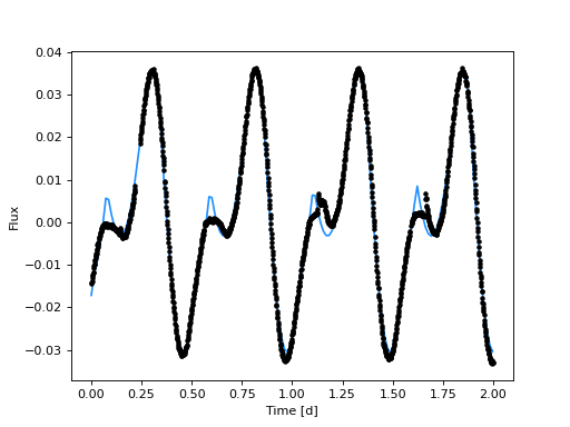
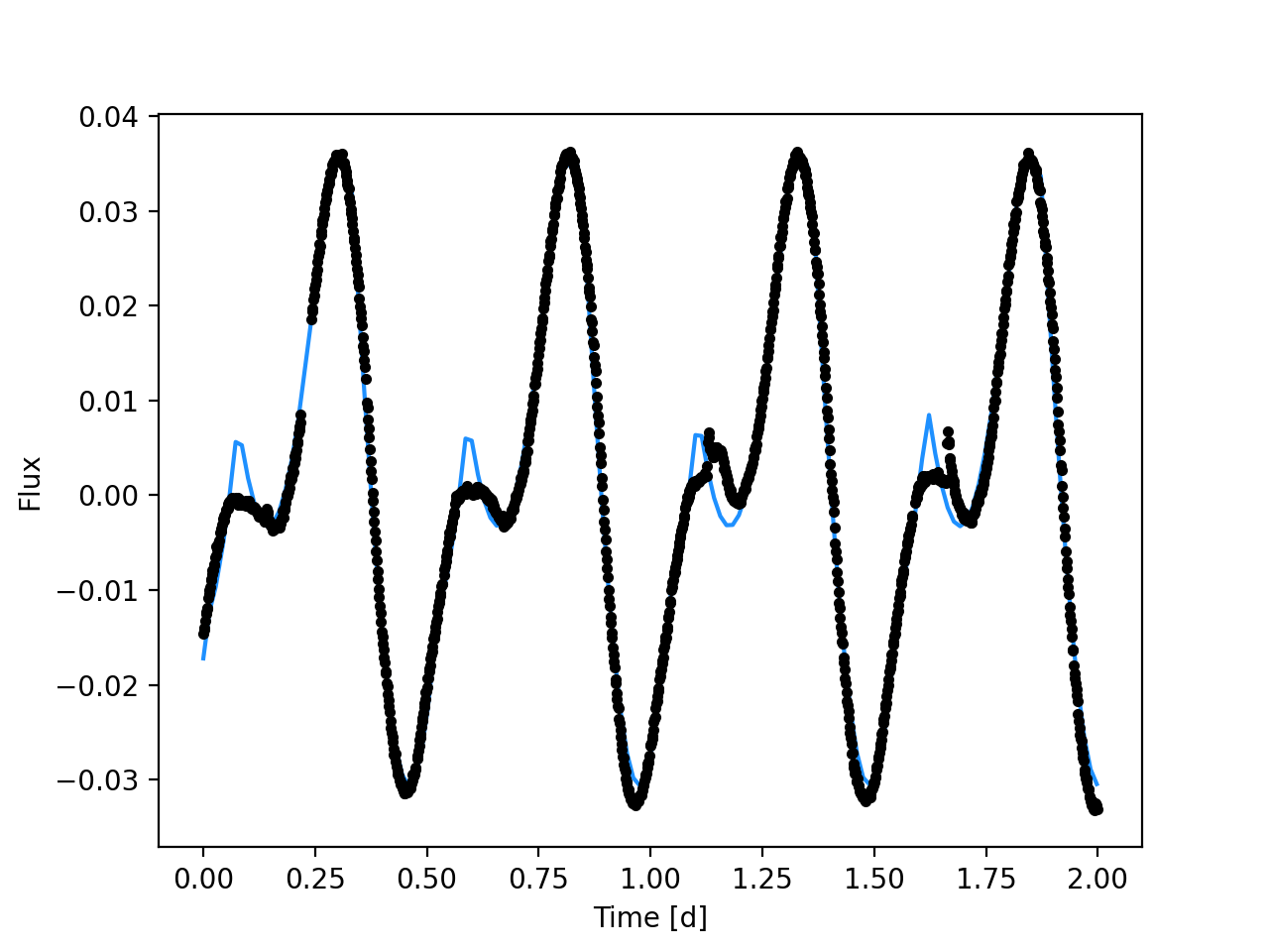
The first thing we should do is check if our model can approximate the data.
Here’s a quick sanity check that our model is defined on the correct bounds,
our errorbar scaling is appropriate, and the number of spots is a good guess,
which we get from running find_MAP which finds the maximum
a posteriori solution:
import pymc3 as pm

with m:
    map_soln = pm.find_MAP()
(Source code, png, hires.png, pdf)

That fit looks pretty good for an initial guess with no manual-tuning and only two spots! It looks to me like the model probably has sufficient but not too much complexity with two spots. Now let’s sample the posterior distributions for the stellar and spot parameters.
Sampling
We’ll sample the posterior distributions using the No U-Turn Sampler (NUTS) implemented by pymc3 by using the normal syntax for pymc3:
import pymc3 as pm

with m:
    trace_nuts = pm.sample(start=map_soln, draws=1000, cores=2,
                           init='jitter+adapt_full')
where we use sample to draw samples from the posterior
distribution. The value for draws used above are chosen to produce quick
plots, not to give converged publication-ready results. Always make the
draws parameter as large as you can tolerate!
The init keyword argument is set to 'jitter+adapt_full', and this is
very important. This uses Daniel Foreman-Mackey’s dense mass matrix setting which is critical for getting fast
results from highly degenerate model parameterizations (like this one).
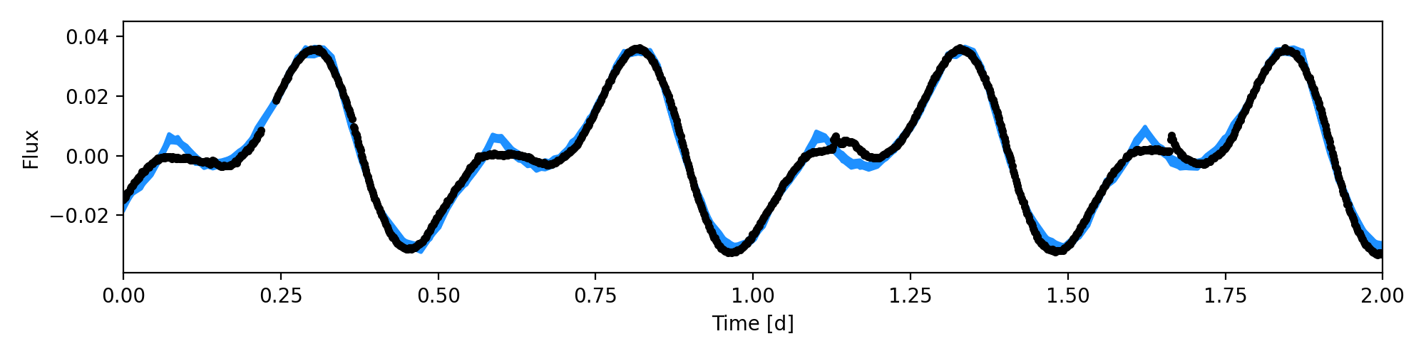
Finally, let’s plot our results:
from dot.plots import posterior_predictive

posterior_predictive(m, trace_nuts, samples=10)
plt.xlim([min_time, max_time])
(Source code, png, hires.png, pdf)
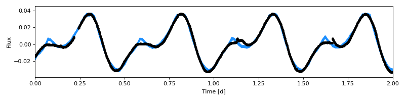
Look at that, the fit is great! Let’s save our model, trace, and summary:
from dot import save_results

results_dir = 'example'  # this directory will be created

save_results(results_dir, m, trace_nuts, summary)
Warning
This tutorial is optimized for producing quick results that can be
rendered online, and does not fully represent best-practices for using
dot. For example, you should make draws as large as you can tolerate
when using dot for science. Ye be warned!